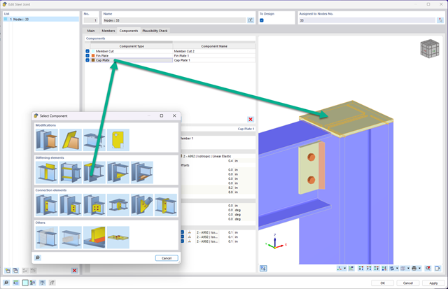
You can now insert a cap plate in steel joints with only a few clicks. You can enter the data using the known definition types "Offsets" or "Dimensions and Position". By specifying a reference member and the cutting plane, it is also possible to omit the Member Section component.
This component allows you to easily model cap plates on column ends, for example.
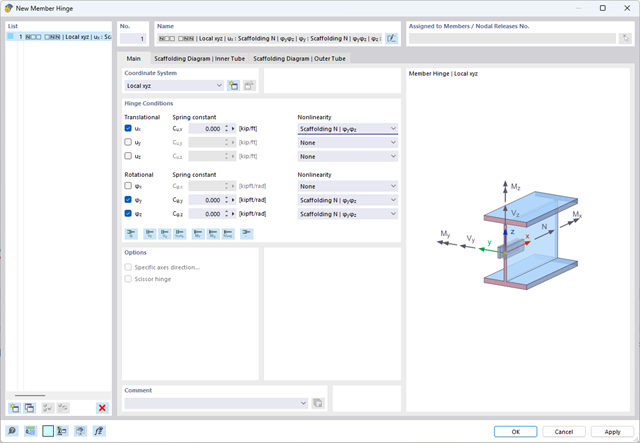
The member hinge nonlinearity "Scaffolding N | phiy,phiz" allows you to simulate an inserted scaffolding tube joint.
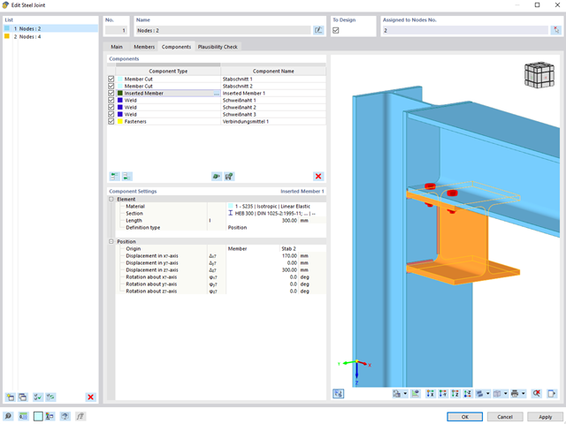
When designing connections, you can now also insert a new member as a component directly in the Steel Joints add-on. This will only be considered for the connection design. You can use the Weld and Fasteners components to connect to other members.
Furthermore, it is possible to use the Member Section and Member Editor components and arrange reinforcement elements on the inserted member, such as stiffeners and tapers.
Go to Explanatory Video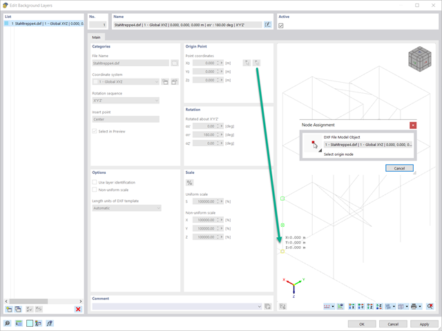
When importing DXF files as background layers, you have the option to select a reference point in the graphic preview.
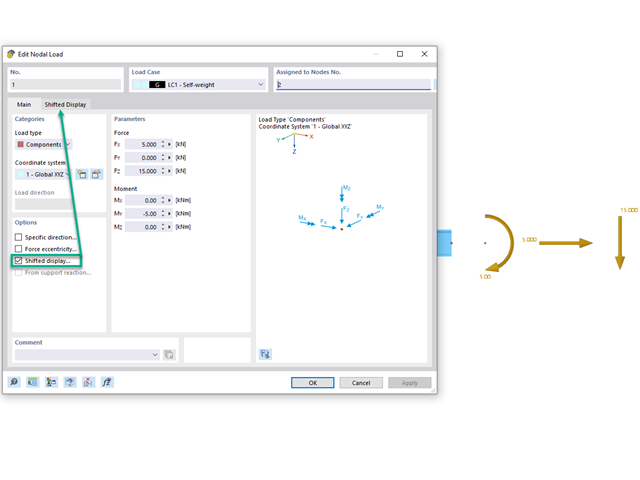
Would you like to display nodal loads or load components that act on one point next to each other? Then use the "Shifted Display" option. This allows you to define offsets in the x, y, and z directions, as well as the size and spacing.
Go to Explanatory Video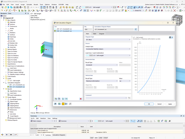
Do you want to create calculation diagrams? With RFEM and RSTAB, this works globally and without any problems. Create and organize your calculation diagrams directly in the Navigator - Data or via the menu Insert → Calculation Diagrams.
Use calculation diagrams to record and display a relation between the various calculation results.
It is also possible to superimpose similar diagrams.
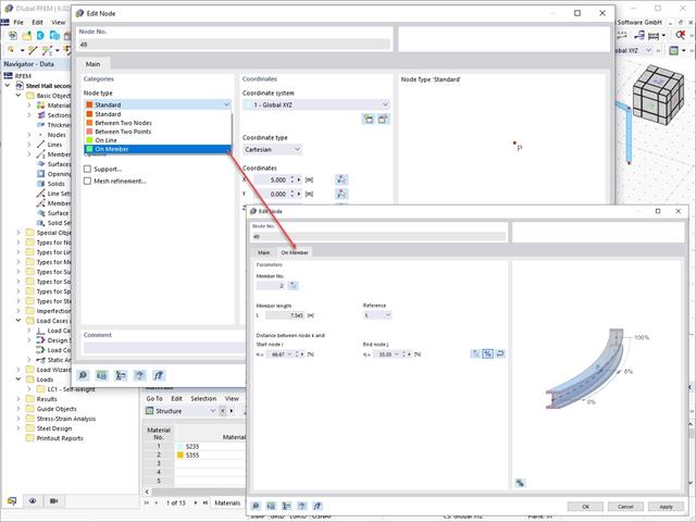
Use the Edit Nodes function to adjust the node type with the automatic specification of all necessary secondary properties. You also have the option to transfer a node to a line or to a member, or to place it between two nodes and two points.

Have you already discovered the tabular and graphical output of masses in mesh points? That's right, this is also part of the modal analysis results in RFEM 6. This way, you can check the imported masses that depend on various settings of the modal analysis. They can be displayed in the Masses in Mesh Points tab of the Results table. The table provides you with an overview of the following results: Mass - Translational Direction (mX, mY, mZ), Mass - Rotational Direction (mφX, mφY, mφZ), and the Sum of Masses. Would it be best for you to have a graphical evaluation as quickly as possible? Then you can also graphically display the masses in mesh points.
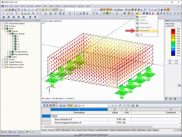
The results of solid stresses can be displayed as colored 3D points in the finite elements.
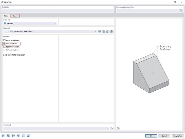
In addition to the "Mesh Refinement" and "Specific Direction" options for solids, you can also activate the "Grid for Results" option, which allows for organizing grid points in the solid space. Among other things, the center of gravity can be set as the origin. There is also the option to activate or deactivate the visibility of the grid for numerical results in "Navigator – Display" under Basic Objects.

Do you want to consider other loads as masses in addition to the static loads? The program allows that for nodal, member, line and surface loads. For this, you need to select the Mass load type when defining the load of interest. Define a mass or mass components in the X, Y, and Z directions for such loads. For nodal masses, you have an additional option to also specify moments of inertia X, Y, and Z in order to model more complex mass points.

Is your goal to determine the number of mode shapes? The program offers you two methods for this. On the one hand, you can manually define the number of the smallest mode shapes to be calculated. In this case, the number of available mode shapes depends on the degrees of freedom (that is, the number of free mass points multiplied by the number of directions in which the masses act). However, it is limited to 9999. On the other hand, you can set the maximum natural frequency the way that the program determined the mode shapes automatically until reaching the natural frequency set.
.png?mw=640&hash=8b43c740f4a91092df759928a6ee21f06f78f8cc)
The calculation of masonry is carried out in compliance with the nonlinear-plastic material law. If the load at any point is higher than the possible load to be resisted, redistribution takes place within the system. This have the simple purpose of restoring the equilibrium of forces. With the successful completion of the calculation, the stability analysis is provided.
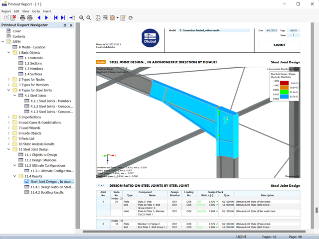
- The results of the connection design can be entered in the printout report
- When creating a new printout report, select the items added from the Steel Joints Add-on
- Use the tool 'Print Graphics to Printout Report' to insert graphics with the results of the connection, including the control panel, into the report
- Printout report contains the specifications of the connection components, design parameters, results and graphics
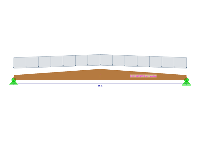
Your options in timber design are diverse. You can consider cut-to-grain angles, transverse tension stresses, and volume-dependent radii of curvature for tapered and curved members. To design the area of the grain cut, the strength is adjusted accordingly in the case of bending tension or bending pressure. In order to also allow you to perform a stability analysis with the equivalent member method, the height to determine the effective and lateral-torsional buckling lengths is set at a distance of 0.65 × h to the actual design point.
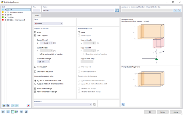
Here you have a free choice. You can perform the support pressure design at any point for the loading in the y- and z-directions of a cross-section. You are free to differentiate between inner and outer supports. A factor kc,90 for the pressure perpendicular to the grain can be user-defined (for example, 1.75 for glued-laminated timber). If allowed, the support length is increased automatically according to the standard specifications. This allows you to achieve a more efficient design with minimum effort.

Did you know that you can also display the moment-axial force interaction diagrams (M‑N diagrams) graphically? This allows you to display the cross-section resistance in the case of an interaction of a bending moment and an axial force. In addition to the interaction diagrams related to the cross-section axes (My‑N diagram and Mz‑N diagram), you can also generate an individual moment vector to create an Mres‑N interaction diagram. You can display the section plane of the M‑N diagrams in the 3D interaction diagram. The program displays the corresponding value pairs of the ultimate limit state in a table. The table is dynamically linked to the diagram so that the selected limit point is also displayed in the diagram.

- Calculation of stationary incompressible turbulent wind flow using the SimpleFOAM solver from the OpenFOAM® software package
- Numerical scheme according to the first and second order
- Turbulence models RAS k-ω and RAS k-ε
- Consideration of surface roughness depending on model zones
- Model design via VTP, STL, OBJ, and IFC files
- Operation via bidirectional interface of RFEM or RSTAB for importing model geometries with standard-based wind loads and exporting wind load cases with probe-based printout report tables
- Intuitive model changes via drag & drop and graphical adjustment assistance
- Generation of a shrink-wrap mesh envelope around the model geometry
- Consideration of environmental objects (buildings, terrain, and so on)
- Height-dependent description of the wind load (wind speed and turbulence intensity)
- Automatic meshing depending on a selected depth of detail
- Consideration of layer meshes near the model surfaces
- Parallelized calculation with optimal utilization of all processor cores of a computer
- Graphical output of the surface results on the model surfaces (surface pressure, Cp coefficients)
- Graphical output of the flow field and vector results (pressure field, velocity field, turbulence – k-ω field, and turbulence – k-ε field, velocity vectors) on Clipper/Slicer planes
- Display of 3D wind flow via animated streamline graphics
- Definition of point and line probes
- Multilingual user interface (German, English, Czech, Spanish, French, Italian, Polish, Portuguese, Russian, and Chinese)
- Calculations of several models in one batch process
- Generator for creating rotated models to simulate different wind directions
- Optional interruption and continuation of the calculation
- Individual color panel per result graphic
- Display of diagrams with separate output of results on both sides of a surface
- Output of the dimensionless wall distance y+ in the mesh inspector details for the simplified model mesh
- Determination of the shear stress on the model surface from the flow around the model
- Calculation with an alternative convergence criterion (you can select between the residual types pressure or flow resistance in the simulation parameters)
- Calculation of transient incompressible turbulent wind flow with the BlueDyMSolver solver
- LES SpalartAllmarasDDES turbulence model
- Consideration of stationary solution as initial state for transient calculation
- Automatic determination of analysis period and time steps
- Use of intermediate results during the calculation
- Organized display of time-varying results via time step units
- Diagram of drag force and point probe results over analysis time
- Display of line probe results for any time steps in a diagram
- Freely adjustable wind permeability for surfaces (Go to Product Feature)
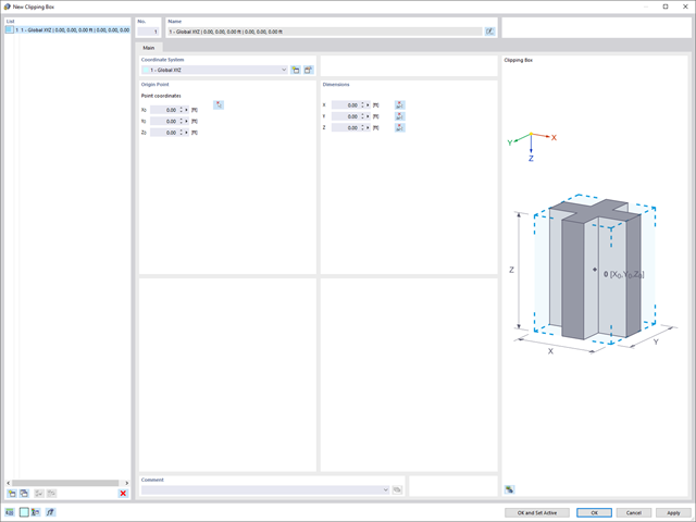
Keep track of what's really relevant to your project. In addition to the clipping plane, you can now define a clipping box. This allows you to hide the irrelevant objects around a focal point.
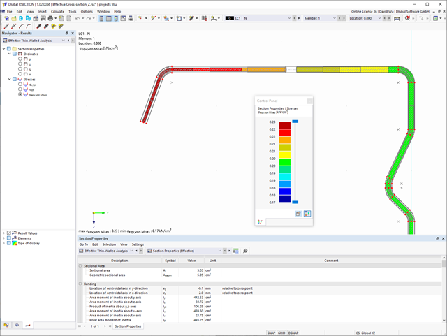
Effective Sections is an extension of the section properties program RSECTION. Compared to the RF‑/STEEL Cold-Formed Sections add-on module for RFEM 5 / RSTAB 8, the following new features have been added to Effective Sections:
- Consideration of the effects of distortional buckling of sections via eigenvalue method
- Definition of stiffeners and buckling panels no longer necessary
- Graphical display of unit stresses
- Optional manual definition of stress points

Compared to the RF-FORM-FINDING add-on module (RFEM 5), the following new features have been added to the Form-Finding add-on for RFEM 6:
- Specification of all form-finding load boundary conditions in one load case
- Storage of form-finding results as initial state for further model analysis
- Automatic assignment of the form-finding initial state via combination wizards to all load situations of a design situation
- Additional form-finding geometry boundary conditions for members (unstressed length, maximum vertical sag, low-point vertical sag)
- Additional form-finding load boundary conditions for members (maximum force in member, minimum force in member, horizontal tension component, tension at i-end, tension at j-end, minimum tension at i-end, minimum tension at j-end)
- Material types "Fabric" and "Foil" in material library
- Parallel form-findings in one model
- Simulation of sequentially building form-finding states in connection with the Construction Stages Analysis (CSA) add-on

Compared to the RF‑/DYNAM Pro - Natural Vibrations add-on module (RFEM 5 / RSTAB 8), the following new features have been added to the Modal Analysis add-on for RFEM 6 / RSTAB 9:
- Preset combination coefficients for various standards (EC 8, ASCE, and so on)
- Optional neglect of masses (for example, mass of foundations)
- Methods for determining the number of mode shapes (user-defined, automatic - to reach effective modal mass factors, automatic - to reach the maximum natural frequency)
- Output of modal masses, effective modal masses, modal mass factors, and participation factors
- Masses in mesh points displayed in tables and graphics
- Various scaling options for mode shapes in the Result navigator

Was your design successful? Then just sit back and relax. You benefit from the numerous functions in RFEM also here. The program gives you the maximum stresses of the masonry surfaces, whereby you can display the results in detail at each FE mesh point.
Moreover, you can insert sections in order to carry out a detailed evaluation of the individual areas. Use the display of the yield areas to estimate the cracks in the masonry.

- Automatic consideration of masses from self-weight
- Direct import of masses from load cases or load combinations
- Optional definition of additional masses (nodal, linear, or surface masses, as well as inertia masses) directly in the load cases
- Optional neglect of masses (for example, mass of foundations)
- Combination of masses in different load cases and load combinations
- Preset combination coefficients for various standards (EC 8, SIA 261, ASCE 7,...)
- Optional import of initial states (for example, to consider prestress and imperfection)
- Structure Modification
- Consideration of failed supports or members/surfaces/solids
- Definition of several modal analyses (for example, to analyze different masses or stiffness modifications)
- Selection of mass matrix type (diagonal matrix, consistent matrix, unit matrix), including user-defined specification of translational and rotational degrees of freedom
- Methods for determining the number of mode shapes (user-defined, automatic - to reach effective modal mass factors, automatic - to reach the maximum natural frequency - only available in RSTAB)
- Determination of mode shapes and masses in nodes or FE mesh points
- Results of eigenvalue, angular frequency, natural frequency, and period
- Output of modal masses, effective modal masses, modal mass factors, and participation factors
- Masses in mesh points displayed in tables and graphics
- Visualization and animation of mode shapes
- Various scaling options for mode shapes
- Documentation of numerical and graphical results in printout report

- Consideration and display of story masses
- Listing of structural elements and their information
- Automated creation of result sections on shear walls
- Output of section resultants in global direction for determining shear forces
- Optional definition of rigid diaphragm by story (story modeling)
- Stiffness type Floor Slab - Rigid Diaphragm
- Defining floor sets,
- for example, calculation of slabs as a 2D position within the 3D model
- Shear walls: Automatic definition of result members with any cross-section
- Design of rectangular cross-sections using the Concrete Design add-on
- Definition of deep beams, design possible using the Concrete Design add-on
- Tabular output of story actions, interstory drift, and center points of mass and stiffness, as well as the forces in shear walls
- Separate result display of the floor and stiffening design
- Free definition of two reinforcement layers
- Design alternatives to avoid compression or shear reinforcement
- Design of surfaces as deep beams (theory of membranes)
- Option to define basic reinforcements for top and bottom reinforcement layers
- Free definition of provided surface reinforcement
- Result output in points of any selected grid
- Design with design moments at column edges
- Determination of deformation in state II; for example, according to EN 1992‑1‑1, 7.4.3, and ACI 318‑19 24.2.3, Table 24.2.3.5
- Considering tension stiffening
- Considering creep and shrinkage
- Fatigue design according to EN 1992‑1‑1, Chapter 6.8 (see this Product Feature)
- Design of a shear joint between the web and flange of ribs
- Optional pure slab or wall design of surfaces for a 2D model type
- Precise breakdown of reasons for failed design
- Design details of all design locations for better traceability of reinforcement determination
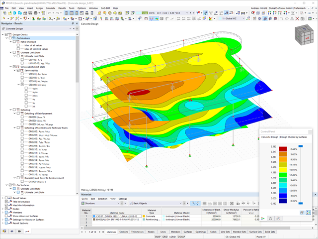
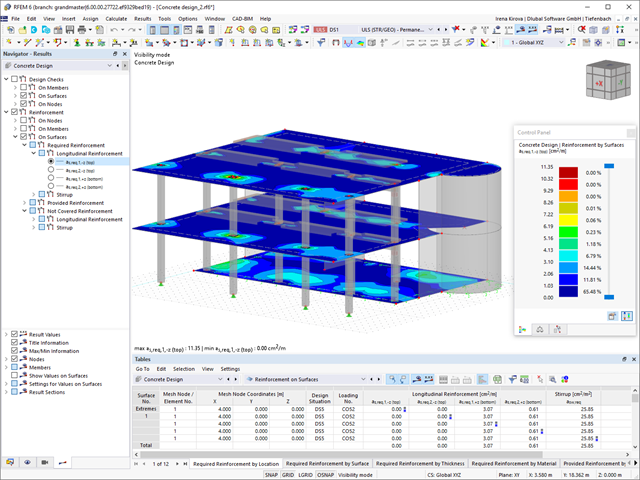
Is the design completed? Then you can lean back. The design ratios of the individual design checks (for example, ultimate limit state, serviceability limit state, or compliance with the construction rules) are displayed for you in a table. You can also find the required reinforcement listed in clearly arranged output tables. The program shows you all intermediate values in a comprehensible manner.
You can display the results of members as result diagrams on the respective member. Furthermore, you have the option to document the inserted reinforcement for longitudinal and stirrup reinforcement, including sketches, in accordance with current practice.
Select whether you want to display the results of surfaces as isolines, isosurfaces, or numerical values. In addition to the design check ratios, you can display the longitudinal reinforcement according to required, provided, and not covered reinforcement.

- Cross-section optimization
- Transfer of optimized sections to RFEM/RSTAB
- Design of any thin-walled section from RSECTION
- Representation of a stress diagram on a section
- Determination of normal, shear, and equivalent stresses
- Output of stress components for the individual member internal force types
- Detailed representation of stresses in all stress points
- Determination of the largest Δσ for each stress point (for example, for fatigue design)
- Colored display of stresses and design ratios for a quick overview of the critical or oversized zones
- Output of parts lists

After you have completed the design, the program takes care of clearly arranged results. Thus, the program shows you the resulting maximum stresses and stress ratios sorted by section, member/surface, solid, member set, x-location, and so on. In addition to the tabular result values, the add-on shows you the corresponding cross-section graphic with stress points, stress diagram, and values as well. You can relate the design ratio to any kind of stress type. The current location is highlighted in the RFEM/RSTAB model.
In addition to the tabular evaluation, the program offers you even more. You can also graphically check the stresses and design ratios on the RFEM/RSTAB model. It is possible for you to adjust the colors and values individually.
The display of result diagrams of a member or set of members enables you a targeted evaluation. For each design location, you can open the respective dialog box to check the design-relevant section properties and stress components of any stress point. Finally, you have the option of printing the corresponding graphic, including all design details.